The Convolution Theorem

The piece studies the Convolution Theorem highlighting its relevance in the resolution of differential and integral equations. It points out that while Laplace transforms of sums of functions is the same as the sum of their transforms, it does not apply to products. Instead, the product of two Laplace transforms is equal to the Laplace transform of convolution of two functions. This is useful especially in determining inverse Laplace transforms, and so solving equations is simple.

 Convolution is defined as a special integral operation on two piecewise continuous functions, expressed as

●        

The properties of convolution mirror those of multiplication:

1.     Commutative:           f * g = g * f

2.     Associative:               f * (g * h) = (f * g) * h

3.     Distributive:              f * (g + h) = f * g + f * h

4.     Zero Multiplication: f * 0 = 0

Convolution is widely applied in engineering, particularly for deriving impulse responses in time-invariant systems. Its commutative property is illustrated in the article, with other proofs left for the reader.

The article discusses the commutative property of convolution along with a proof, example, and remarks on the theorem of convolution.

Key Points:

1.     Commutative Property of Convolution:

○      The property states that the convolution of two functions, f * g, is equal to g * f.

○      Proof:

■      The proof involves a change of variable from τ to v = t - τ in the convolution integral:
(f * g)(t) =
               =

■      By definition, this is equal to (g * f) (t), proving the commutative property.

2.     Example:

○      To verify the property, the convolutions (t² * sin t) and (sin t * t²) are computed using their respective integral definitions. Both yield the same result, confirming the commutative nature of convolution.

○      Additionally, the example demonstrates that one computation might be simpler than the other, depending on the setup.

3.     Convolution Theorem:

○      Statement:

■      If L{f(t)} = F(s) and L{g(t)} = G(s), then:
L⁻¹{F(s)G(s)} = (f * g)(t)

○      Proof:

■      It starts with the Laplace transform of a convolution:
L{(f * g)(t)} = ∫₀⁺∞ e^(-st)(f * g)(t)dt

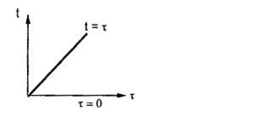
■      Substituting the convolution definition and rearranging the region of integration lead to the result aligning the Laplace transform of a convolution to the product of their individual Laplace transforms.

Significance:

·        Convolution integrals computations are greatly simplified by commutative property.

·        With the aid of the convolution theorem, differential equations and inverse transforms are much easier to tackle which helps in deep engineering and analytical math.

The convolution theorem is extremely helpful when it comes to solving problems concerning the Laplace transform, as well as aiding greatly in the inversion of Laplace transformations. Here’s a brief description of theory together with proof and illustrations:

Key Concepts:

1.     Statement of the Convolution Theorem:

○      If L{f(t)} = F(s) and L{g(t)} = G(s), then:
L{(f * g)(t)} = F(s)G(s)

And inversely:
L⁻¹{F(s)G(s)} = (f * g)(t)

Proof Steps:

1.     Primary Proof:

○      Start with the Laplace transform of the convolution:
L{(f * g)(t)} =

○      Substitute the convolution definition and change the order of integration.

○      Rearrange into two nested integrals, factor terms, and simplify, arriving at:
L{(f * g)(t)} = F(s)G(s).

2.     Alternate Proof:

○      Compute the product of two Laplace transforms directly, F(s) G(s), using their definitions.

○      Swap integration order and apply the variable substitution t = u + v.

○      This reformulation also leads to F(s) G(s) = L{(f * g)(t)}.

Examples Highlighting Applications:

1.     Convolution of Trigonometric Functions:

○      Example to compute (cos(at) * sin(at)) as a convolution integral:
(cos(at) * sin(at)) = ∫₀ᵗ cos(aτ)sin(a(t-τ))dτ

○      Using trigonometric identities and integration yields:
(cos(at) * sin(at)) = ½t sin(at).

2.     Finding an Inverse Laplace Transform:

○      To compute L⁻¹{2/(s²(s² + 1))}, direct partial fraction decomposition proves cumbersome.

○      Instead, apply the convolution theorem:
L⁻¹{2/(s²(s² + 1))} = 2(L⁻¹{1/s²} * L⁻¹{1/(s² + 1)})
                      = 2(t * sin(t)).

○      Expanding and solving the convolution integral produces the result:
2(t - sin(t)).

Significance and Applications:

●      The convolution theorem simplifies otherwise complex computations, such as evaluating inverse Laplace transforms without resorting to partial fraction decomposition.

●      Useful in solving differential equations, systems in engineering, and deriving system impulse responses.

●      Convolution provides an efficient mathematical framework for real-world applications, particularly in signal processing and control systems.

By showcasing both proof approaches and practical examples, the convolution theorem is demonstrated as a powerful mathematical tool for simplifying and solving advanced problems efficiently.